In this section, we explain how to use the Conley-Morse Database code (CMD) on a single computer with a fixed set of parameters.
For each dynamical system, one creates a subdirectory which should contain three files : Model.h, ModelMap.h, and config.xml. The examples provided with the source code are located in the subdirectory examples/. For simplicity, one could simply copy and paste the files included in the subdirectory examples/Leslie2D/ which are fully commented and should be fairly easy to modify.
To explain the procedure on how to set up the model and use the code, we will use the files in the subdirectory examples/Leslie2D/ which implement the Leslie population model.

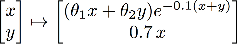
We will restrict the two dimensional phase space to [ 0.0, 320.056 ] x [ 0.0, 224.040 ] with parameter values θ₁ = 26 and θ₂ = 22.7.

Step 1 : Setting up the dynamical system

The file config.xml defines all the values necessary to run successfully CMD. Since we are using the markup language xml, fields are given between tags of the form <tag> ... </tag> and within its tags particular option values are given between two tags of the form : <option> value </option>. Prior knowledge of xml is not necessary, and we describe below the different section of the file config.xml.
The file config.xml should always start with <config> and end with </config>. Within these two tags, we will include different fields and values that are necessary to run CMD.
The first field that can be given is a name as well as a short description for the model:

<model>
  <name> Leslie2D </name>
  <desc> Two dimensional Leslie model </desc>
</model>

The information regarding the parameter space is given within <param> ... </param>. We first enter the dimension of the parameter space or the number of parameters in the problem, in our case 2. For each parameter we can enter the range of values they can take. Each parameter range will be subdivided and the Conley-Morse Database code can use at runtime any of these subintervals for the computation of the map.
The last option that can be entered is the number of subdivisions for each parameter range. In our case, this value is ignored since the lower and upper bounds are the same.
A snippet of the code is

<param>
  <dim> 2 </dim>
  <bounds>
    <lower> 0.0 0.0 </lower>
    <upper> 50.0 50.0 </upper>
  </bounds>
  <subdiv>
    <depth> 5 </depth>
  </subdiv>
</param>

We give the information regarding the phase space within the tags <phase> ... </phase>.
We first enter the dimension of the phase space, which is 2. The lower bound of the phase space in each direction 0.0 and the upper bounds of the phase space are 320.056 224.040.
In order to construct the Morse sets, the phase space will be divided successively along each direction. For an initial stage, we subdivide every grid element unconditionally for a prescribed number of times. At each further stage of subdivision recurrent sets are calculated and only they are flagged for further subdivision. Subdivision stops when certain criterion are met which we may configure. The configuration involves four integer settings which we call "init", "min", "max", and "limit". The "init" setting is the number of subdivisions in the initial stage. The latter settings tell us when to stop the subdivision of recurrent sets. In particular we do not stop subdividing until one of two criterion are met: either (1) the subdivision level is deeper than "min" and has more than "limit" grid elements, or (2) the subdivision level is "max". The purpose of these rules is to allow us to robustly deal with a phenomenon of "spurious" Morse sets that may appear; further subdivision may make them disappear, but we do not want to waste time subdividing large Morse sets deeper than the "min" level.

<phase>
  <dim> 2 </dim>
  <bounds>
    <lower> 0.0 0.0 </lower>
    <upper> 320.056 224.040 </upper>
  </bounds>
  <subdiv>
    <init> 0 </init>
    <min> 24 </min>
    <max> 28 </max>
    <limit> 1000 </limit>
  </subdiv>
</phase>

The file Model.h defines the parameter space, phase space, and the map. See that for the map, it produces a Map object defined in ModelMap.h. In fact the Model.h file from Leslie2D is likely to be suitable for many different Models, and all that would need to be done is to replace ModelMap.h with different code.

Step 2 : Compile and run

The SingleCMG program can be compiled and run as follows:

 cd conley-morse-database
 make SingleCMG MODELDIR=./examples/Leslie2D
 cd ./examples/Leslie2D
 ./SingleCMG ./ 20 20

This program analyzes a single parameter box. The first argument is the path to search for the ./config.xml file. The latter two are the parameter values (Leslie2D has two parameters). We can give intervals as parameters instead of exact values if we give four parameters. In this case the first set of parameters is treated as lower bounds and the second set as upper bounds. For example, the following indicates to do the calculation over the parameter box [19.0,20.0]x[20.0,21.0]:

 ./SingleCMG ./ 19.0 20.0 20.0 21.0  

To run the full database program on a cluster, a scheduler submission script is necessary. We have provided an SGE script which we use; for non-SGE schedulers or simply to fine-tune the scheduler settings (in particular the number of processors) the "script.sh" file should be modified. Once this is done, it should suffice to type:

 cd conley-morse-database
 ./CMDB ./examples/Leslie2D

The conley-morse-database program can also be executed on a single computer with Open-MPI installed:

 cd conley-morse-database
 make MODELDIR=./examples/Leslie2D
 cd ./examples/Leslie2D
 mpiexec -np 8 ./Conley_Morse_Database ./

This is probably only suitable for testing or very small databases.

Step 3 : Interpretation of the SingleCMG results

By default, the CMD code will output three bitmap images in the model directory. The first image grid.bmp represents the different level of subdivisions of the phase space in gray scale, the darker the deeper/finer the grid. The second image morse_sets.bmp depicts the Morse sets found. This image just encloses the Morse sets and is a subregion of the phase space. The last image is grid_and_morse.bmp which is simply a composition of the first two images and allow to see where the Morse set are located in the phase space. Below are the images obtained from the Leslie model with the set up described on this page.

grid.jpg	morse_sets.jpg	grid_and_morse.jpg

The Morse graph is given in the file morsegraph.gv which can be opened with the software graphviz. Below is the morse graph from the Leslie model and each Morse set is labelled with its Conley Index.

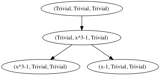
For interpretation of the Conley_Morse_Database results, see the Database Explorer page.