The user interface of the explorer has 4 components:
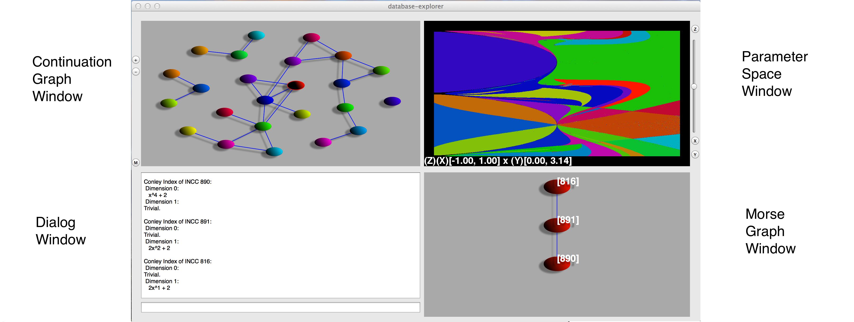
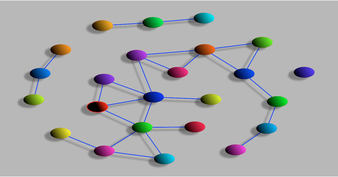
The upper left window exhibits the continuation graph, which is a representation of parameter space of the database. Each vertex corresponds to a Conley-Morse graph continuation class and thus contains two pieces of information: a Conley-Morse graph and the collection of grid elements in parameter space for which this Conley-Morse graph describes the global dynamics. Each edge in the continuation graph indicates which vertices contain adjacent parameter boxes.
Depending on the system the number of nodes in the continuation graph can be quite large. To make interpreting the graph feasible we order the continuation class by the number of grid elements they contain. By default the 10 largest continuation classes are shown. The +/- toggle keys on the left hand side of the explorer allow the user to increase or decrease the number of visible vertices. Some vertices may appear to be disconnected from the rest of the graph, which typically indicates that the adjacent vertices are too small to be visible.
The M button to the left of this window will highlight every continuation class with multiple basins of attraction, as indicated by more that one minimal Morse node in the Morse graph. A warning: this button will only highlight continuation classes already visible in the continuation graph.
The upper-right window of the database explorer provides an interactive picture of a two-dimensional slice of parameter space. At the bottom of this window is a description of the range of parameter space as a product of intervals. The order of these intervals is the same as their order in the database computation. Each continuation class is represented by a different color.
If parameter space is two-dimensional, this is a complete picture. If parameter space is more than two-dimensions, the explorer allows the user to display any two dimensional slice defined by two parameter values. This is done using the x,y,z toggle keys at the bottom of the window and the slider at the right of the window. To choose a parameter to be the x-axis, hit the x button until the (X) is displayed before the desired interval. The same process with the y button sets the y-axis. To control the choice of the other parameters, use the z button to first select which parameter you want to set then move the slider to choose the value for that parameter that you want.
To zoom in on a particular region, simply click and drag a window on the region you want to zoom in on. To zoom back out, double click anywhere in the frame.
The lower-right window of the database explorer displays the Hasse diagram for the Morse graph of a given continuation class. The edges should be interpreted as arrows pointing downward.
Each Morse node is labeled by the number of its Isolating neighborhood continuation class.
This window can be used to discover the following information:
As an example we will demonstrate how one can use the database explorer with the file newton-2-10-12.cmdb. For more other database computations you can go here. To load the file into the explorer open the program and a prompt will automatically be displayed allowing you to choose which file to open. Upon loading the database, the explorer should look like Figure 1. Note that the colors are generated at random, so the picture you see may not be identical but the shapes of the regions in the parameter space window should be.
The continuation graphs in Figures 1 and 2 have 24 vertices, but the default number shown when the explorer opens is 10. To increase the number of vertices hit the + key on the left side of the explorer. Each vertex corresponds to a contiguous region in the parameter space window of the same color. To highlight the corresponding region simply click on the vertex. Information about the continuation class will also be given in the interactive dialog when you do this. For example, you might see:
Size of MGCC 492: there are 24548 parameter boxes
This says that the node you clicked on has been designated Morse graph continuation class (MGCC) number 492, and tells you the number of parameter boxes in that class.
One can also select a particular continuation class by clicking in the parameter space window. The region selected will be highlighted in the parameter space window as will the corresponding vertex in the continuation graph. One difference when clicking on parameter space instead of on the continuation graph is what appears in the dialog window: instead of information about the total number of parameter boxes in the continuation class, the specific numerical values defining the parameter box you clicked on will be displayed.
Clicking on a vertex in the continuation graph or in the parameter window also produces the Morse graph for that continuation class to appear in the Morse graph window. The Morse graph, in conjunction with the Conley index information at each node, summarizes the dynamics that are stored in the database for each parameter box.
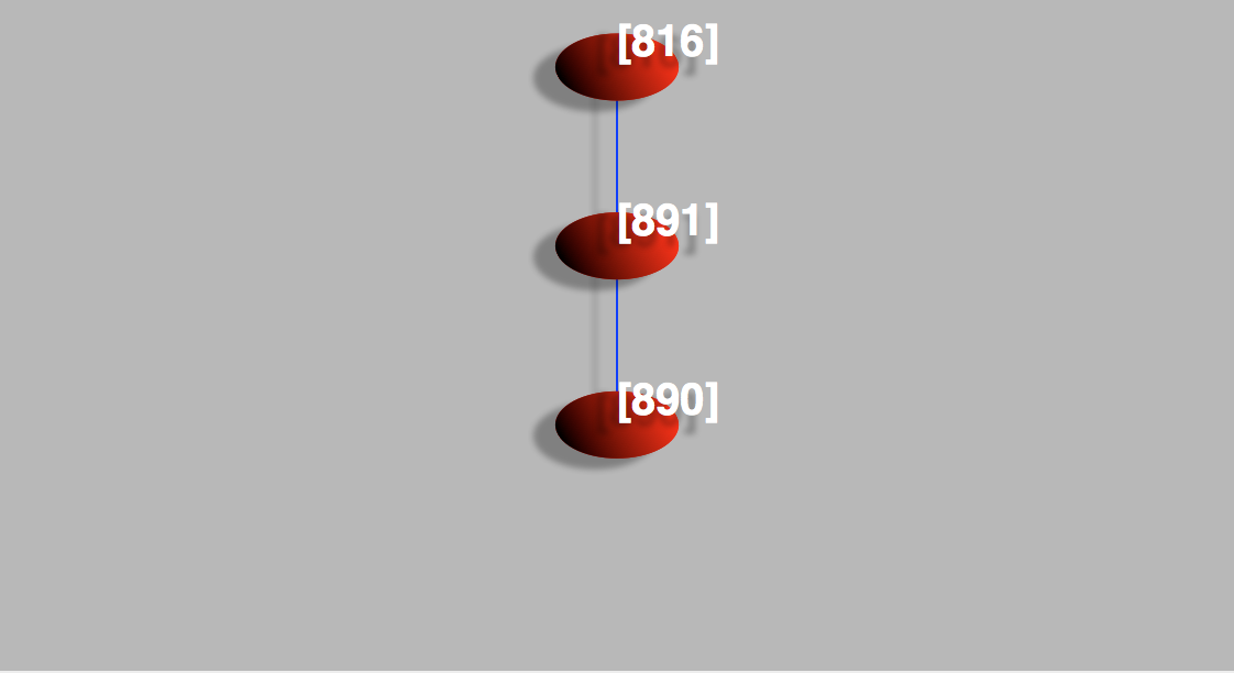
In the case of Morse graph continuation class 492 (representing the bright red region in Figure 3) we see that the Morse graph (Figure 4) consists of three Morse nodes, each representing recurrent dynamics found by our algorithms in the given region of parameter space. Each node is labeled by a number: in this case 816, 891, and 890. Furthermore, the Morse nodes are arranged in a directed graph, where the edges in the Morse graph window are understood to point downwards. This directed graph is the Hasse diagram of the partial order on the Morse nodes If there is no path between two Morse nodes then this is a theorem that there is no trajectory in the dynamical system between the two. For example, there is no trajectory from Morse node 891 to Morse node 816 because the latter is higher in the partial order. On the other hand, the converse does not hold in general: the existence of an arrow from Morse node 816 to Morse node 891 does not guarantee the existence of such a trajectory in the underlying system. Such "false positives" can occur as a result of the discretization used in the computation.
In addition to the ordering the Morse nodes given by the Morse graph, the database stores the Conley index of each Morse node which gives information about the dynamics that occur within each Morse node. To get the Conley index of a particular Morse node, simply click on it inside the Morse graph window and the Conley index information will appear in the Dialog window. As an example, if we click on Morse node 890 we get the following:
Conley Index of INCC 890:
Dimension 0:
x^4 + 2
Dimension 1:
Trivial.
The presence of Conley index on dimension 0 here indicates stable dynamics, as one would expect from a minimal node in the partial order. The coefficients used to compute this particular database were taken mod 3, so the polynomial x^4 + 2 is congruent to x^4 - 1. By definition, a Morse node with this Conley index in dimension 0 is a stable 4-cycle set, meaning it has robust period-4-like behavior for every parameter value in this Conley-Morse graph continuation class.
One small detail that should be mentioned: INCC stands for Invariant neighborhood continuation class. This is defined so that any two Morse nodes (perhaps from different Conley-Morse graph continuation classes) in the same INCC provably have the same Conley index. It is possible that two Morse nodes in the same Conley-Morse graph continuation class have the same INCC, in which case the INCC would not uniquely identify the Morse nodes in the Morse graph.
If we click on Morse node 891 we get the following Conley index information:
Conley Index of INCC 891:
Dimension 0:
Trivial.
Dimension 1:
2x^2 + 2
Here the absence of any dimension 0 Conley index indicates unstable dynamics. The dimension 1 Conley index of 2x^2 + 2 = x^2 + 1 (mod 3) is suggestive of unstable period 2 dynamics with an orientation reversal.
Morse node 816 has the following Conley index:
Conley Index of INCC 816:
Dimension 0:
Trivial.
Dimension 1:
2x^1 + 2
This is, again, unstable dynamics, although in this case the Conley index x+1 is suggestive of an unstable, orientation-reversing fixed point.
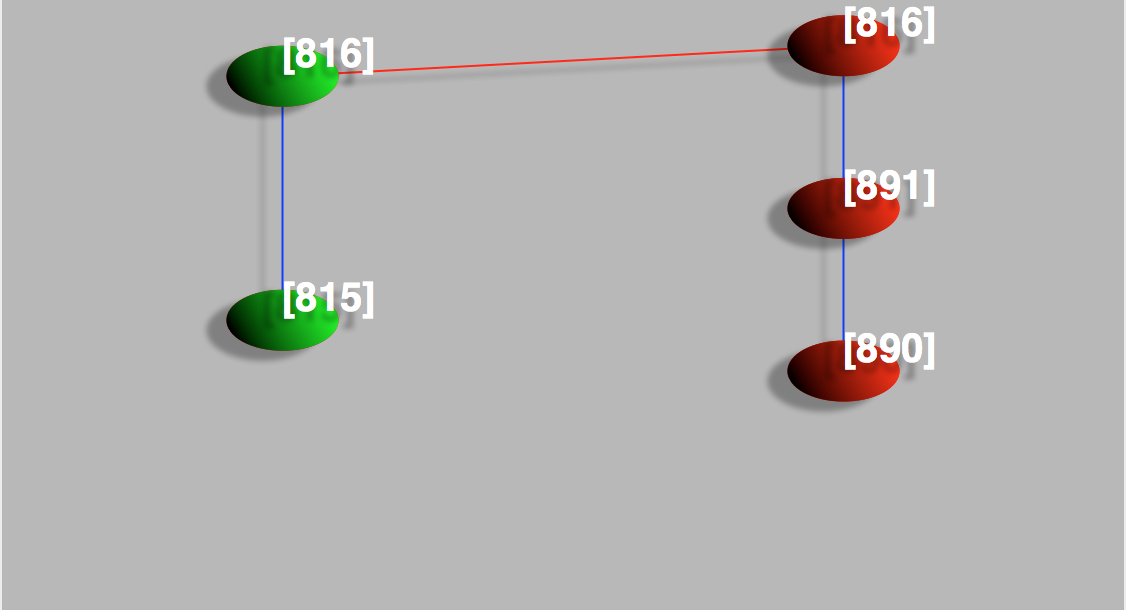
The Conley-Morse graph continuation classes represent the set of parameter boxes over which this stored information about the dynamics—both the partial order of Morse nodes and the Conley index information—provably extends. But in some cases one might want to know more about the parameters over which dynamics for one particular Morse set provably extends without being concerned about the global dynamics extending—by definition this is the Invariant neighborhood continuation class. The command line in the dialog box is designed for these type of queries. For example, if one is interested in parameter boxes with dynamics that can provably be continued from Morse set 816, one can enter 816 into the command line and hit 'return'. The set of vertices in the continuation graph containing this INCC will be highlighted in red boxes.
To see how the Morse sets continue between neighoring continuation classes one can click on the edges in the continuation graph. Figure 5 shows an example of the Morse graph window after doing so. Here the green Morse graph represents the large green region in Figure 3 adjacent to the bright red region. As you can see, both regions contain INCC 816 (also indicated by the red line joining the two Morse sets) representing the same unstable dynamics discussed above. The two continuation classes are distinct however, because the global dynamics does not continue: in the green region only a 2-cycle set (INCC 815) is guaranteed to be observed instead of a 4-cycle set.
Because of its usefulness in applications, a similar query for the Conley-Morse graph continuation classes with multiple attractors (i.e. multiple minimal Morse nodes) is implemented as the M button on the left side of the explorer. After pressing the M button all vertices representing classes with multiple attractors are highlighted in red.
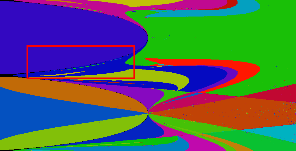
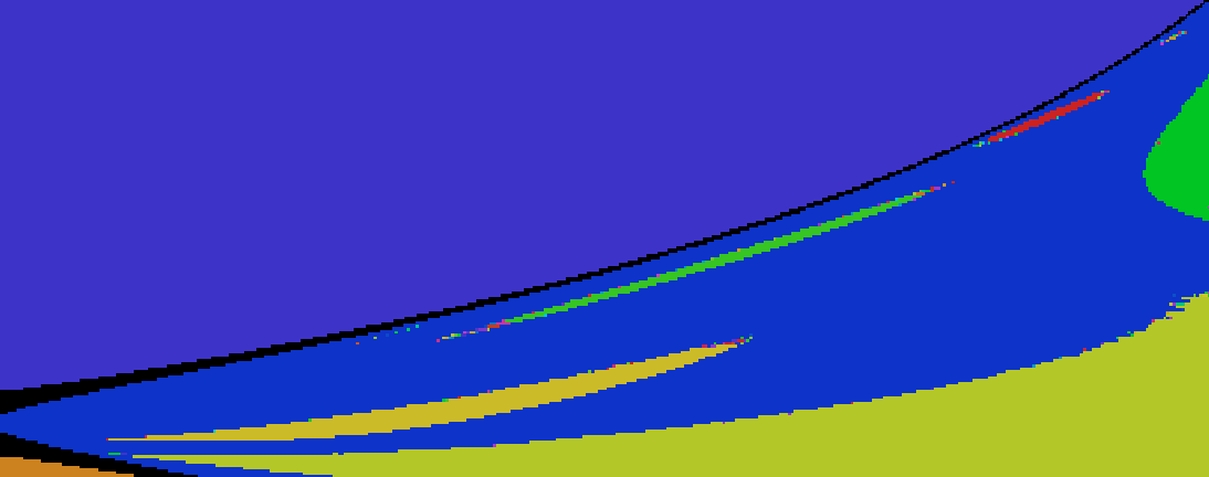
Finally, especially in cases where parameter space is finely subdivided, there may be details in the parameter space window that one wants to magnify. Clicking and dragging a rectangle over the desired region in parameter space will zoom in on that location. By zooming in on the region indicated in FIgures 6 and 7 we can find Morse graph continuation classes with Morse nodes that exhibit an attracting 9, 11, and 13-cycle sets. These are the thin slivers in Figure 7, with periods increasing as you go up and to the right.