Work done by Miro Kramar^†, Arnaud Goullet^†, Lou Kondic^‡, Konstantin Mischaikow^†

† : Rutgers University, NJ ‡ : New Jersey Institute of Technology, NJ

With the goal of extending our ability to systematically explore network properties in greater detail, we developed rigorous mathematical models capable of capturing geometric features of  particle interactions. The approach  is based on algebraic topology and in particular persistent homology.  This is  a relatively new mathematical technique that provides a computationally efficient rigorous framework for  multi scale analysis. The computational efficiency is essential since the goal is to apply these techniques to large data sets. Persistent homology reduces a scalar function to a persistence diagram, which is a collection of points in the plane where each point encodes well defined geometric information about the function, but does not rely on a particular choice of threshold to do this.  In the context of particulate systems, this means that a  specific definition of `force-chains' or similar objects is not required. Furthermore, there are a variety of metrics that can be imposed on the space of persistence diagrams such that in the context of particulate systems the application of persistent homology can be interpreted as a continuous non linear projection of the force networks to the space of persistence diagrams. These properties of persistent homology suggest that it is a good tool to study both the static and  the dynamical aspects of experimental and computational realizations of particulate systems.

As indicated above, persistent homology is based on algebraic topology and thus its computation is based on the construction of a finite complex.  The construction of appropriate complex depends upon the type of data that is provided, which in turn is dependent upon the method by which the data is obtained. We propose three different complexes: digital,  position, and  interaction.  The information that can be extracted via the use an interaction network is significantly more reliable than that of a digital or position network.  The interaction network can be used in the setting of numerical simulations or particular types of experiments where complete information about the  forces between adjacent particles may be known. However, for many experiments only the total force experienced by a particle may be available.  This necessitates the use of a digital or position network, depending upon how the data is collected and physical properties of the individual particles.

Different networks

Interaction network	Position network	Digital network

The interaction and position network can be interpreted as a real valued function on a simplicial complex. In case of the digital network the function is defined on a cubical complex which corresponds to pixels or voxels.

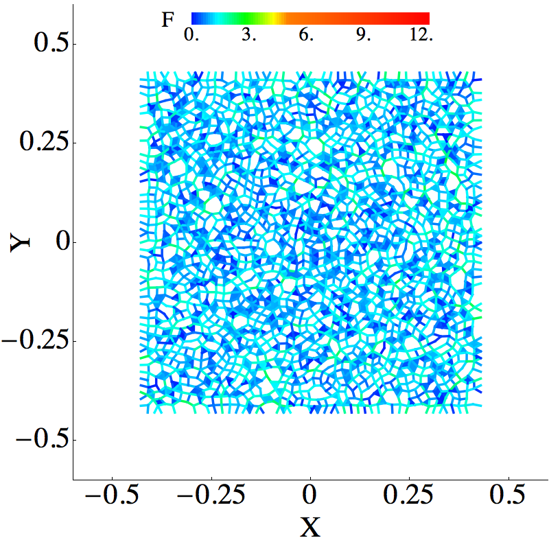
Interaction network

The underlying simplicial complex for the interaction network is a full 2 dimensional  or 3 dimensional complex with vertices corresponding to the particles. It is every edge between any two vertices, every  triangle and possibly tetrahedrons are present. The definition of the function is derived from the inter particle  interactions. In our case the value of the function on the edge between two particles is a magnitude of the normal force acting between these particles. In order to extend this function to all simplecies  we use the following procedure. The value at a vertex is a maximum over the edges that contain the given vertex. The value on two and tree dimensional simplecies is a minimum of the edges contained in the closure of the simplex.

Position network

The underlying simplicial complex for the position network is a 2 dimensional  or 3 dimensional complex with vertices corresponding to the particles. The edge between two vertices is present if the particles are in contact. The higher dimensional simplex is present if all its edges are present. The definition of the  function derived from the knowledge of some quantity assigned to the particles. In our case this quantity is the magnitude of total normal force experienced by the particles. Again the function is extended to higher dimensional simplecies by taking a minimum over the edges that are contained in their closure.

Digital network

The digital network can be constructed from a digital image by assigning the values of the pixels to the 2D dimensional cubes. Tho extend the function to the edges and vertices a minimum over the cubes containing the particular edge or vertex is taken.

Code for constructing the networks and computing their homology.

Persistent homology of the interaction network

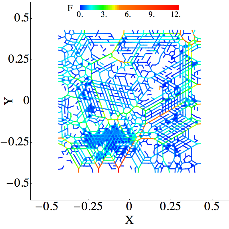
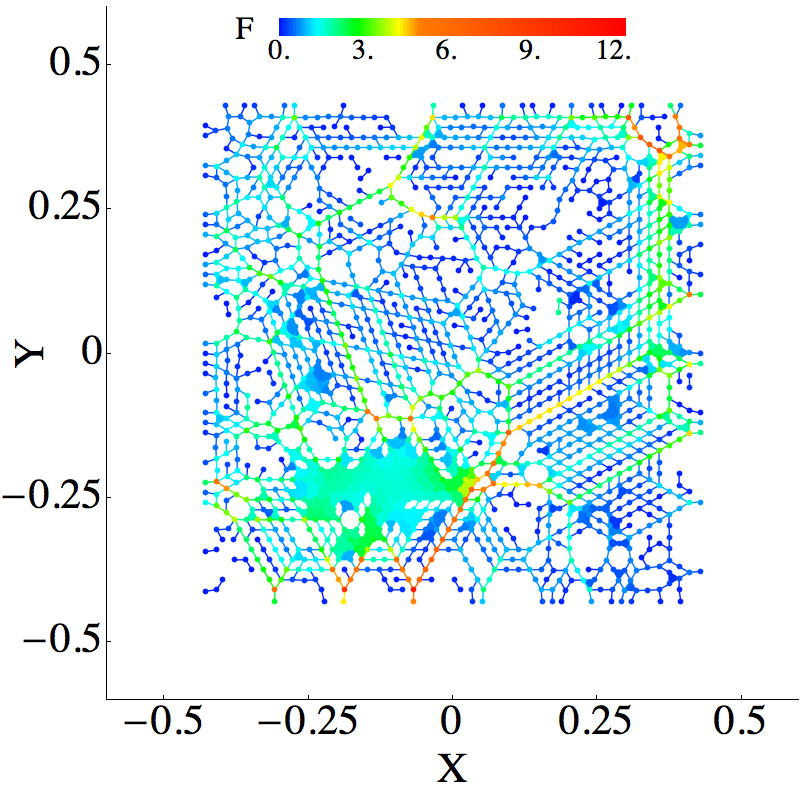
To demonstrate the power of persistence diagrams we use them to compare mono disperse frictionless system with poly disperse system with friction. Both systems are at the onset of jamming.

Mono disperse system without friction
Poly disperse system with friction

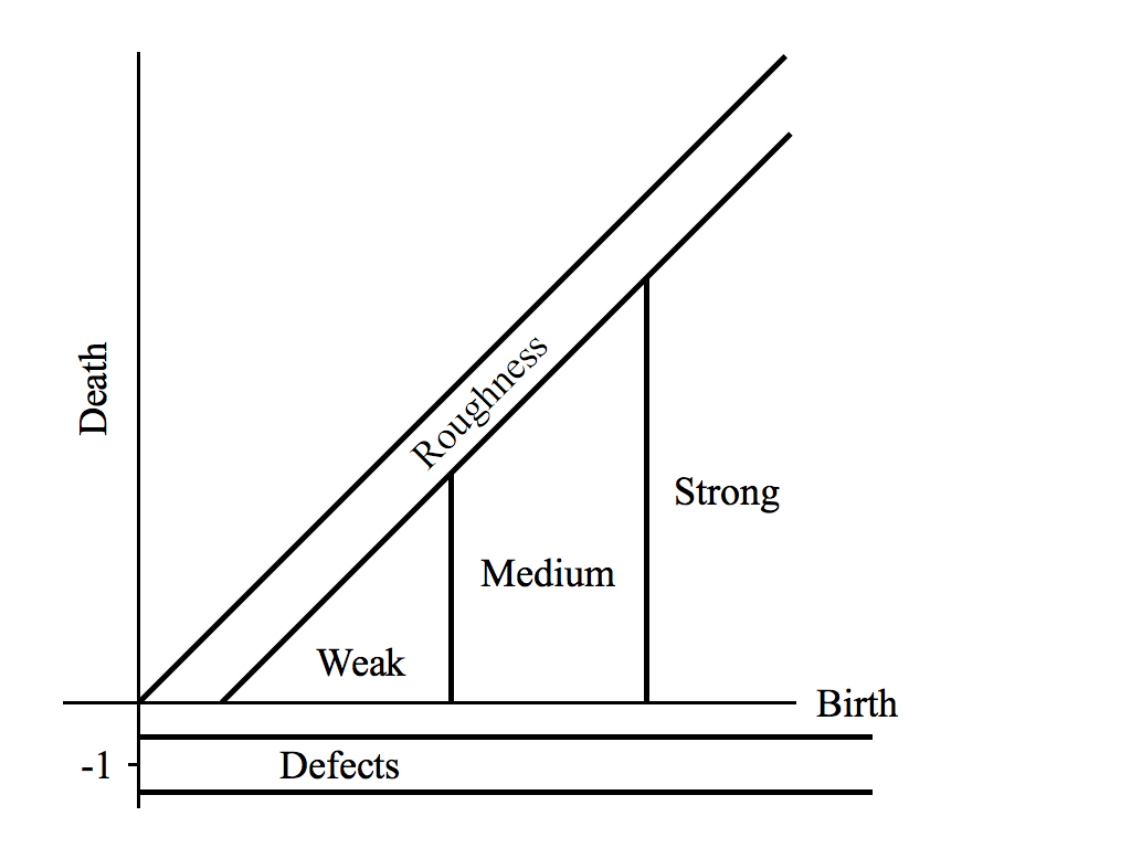We begin by assigning  physical meaning to the location of persistence points in the persistence diagrams. Figure on the laft shows a persistence diagram divided into five regions. With the exception of the region labelled defects, the location of the division lines is intended to be either  system specific or  conceptual.  We explain these divisions in the context of the interaction force networks and persistence diagrams of the shown above. A more complete analysis of DGM using these ideas is presented in our paper.

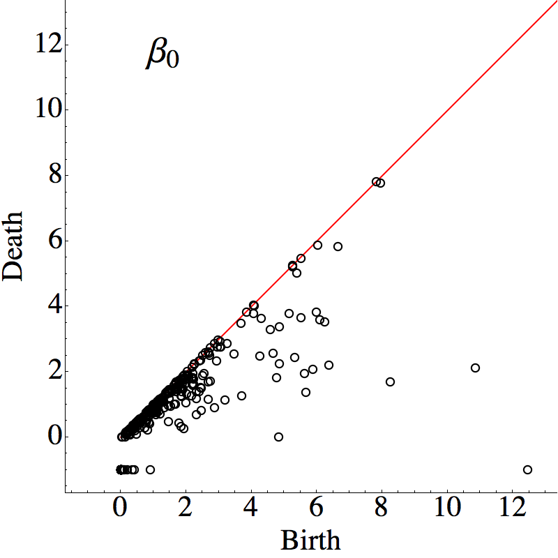
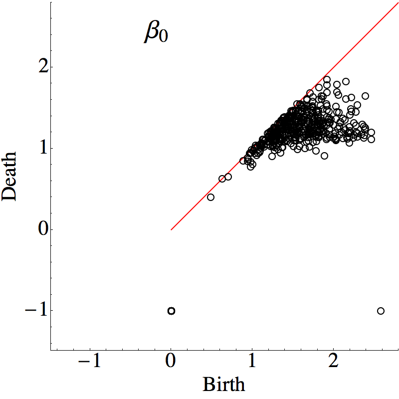
There are at least two different interpretations of the points in the 0-dimension persistence diagram that lie close to the diagonal; the region we have labelled as roughness. The first is to treat this as noise, i.e. a byproduct of the imperfect  measurements of the normal forces between particles. While this may be appropriate for many experimental settings, the data  represented here comes from numerical simulations.  Thus, the errors are extremely small compared to the size of the normal forces. This leads to the  second interpretation, which we adopt, that this region of the persistence diagram provides a measurement of how rough or bumpy the normal force landscape is, e.g. should we view the surface of the landscape as being made of glass or sandpaper? Alternatively, the points in the 0-dimension persistence diagram that lie outside the roughness region provide a means of  measuring how non-uniform the normal force landscape is. Therefore by comparing  the diagrams for the mono disperse frictionless system and poly disperse system with friction we  conclude that the landscape of the poly disperse system is rougher .

To understand the region labelled as strong, observe that the image of the interaction network for poly disperse system does not contain any red simplices, implying that there are no extremely strong force interactions.  In contrast, such red simplices are present in the mono disperse system. This difference can be inferred from the 0-dimension persistence diagrams. The value 1 represents the average interaction force. For the poly disperse system there are no persistence points with the birth value larger than 3 and only a few points with birth value larger than 2.5.  Thus, depending on the exact cut-off there are no or at most few points in the region marked strong for the poly disperse system system, in clear contrast to the mono disperse system. 
If we take the left division marker for the medium regime to be 1, then the persistence points in the moderate and strong regions provide information about the geometry of what the DGM community typically refer to as a force chain. In the case of  the poly disperse system, we see a large number of points in the 0-dimension persistence diagram  that are born between 1 and 2.5 and die before 0.8. This suggests a landscape consisting of moderately high peaks separated by moderately high valleys.  To continue the geographic metaphor, the  interaction network of poly disperse system takes place on a high plateau. In contrast,  the mono disperse system has fewer moderately high peaks, but they are separated by much deeper valleys since there are points with death values below $0.6$.   Therefore, we conjecture that  the  landscape for the mono disperse system has fewer peaks (but some of them are strong) than that of the poly disperse  system, and these peaks are  in general much more isolated and more likely to be separated by valleys of much weaker forces.

Finally, we consider the region labelled defects.  In a 0-dimension persistence diagram each point in this region  corresponds to a distinct connected component.  In the context of the poly disperse  system these mostly correspond to rattlers.  This conclusion is obtained by observing that aside from the single persistence point with a large birth force, that corresponds to the component containing most of the particles, the persistence points in the defects region have a birth value of 0, indicating that they are not experiencing any normal force.  This is quite different from the mono disperse system. In this case we have persistence points in the defects region with non-zero birth forces. This implies the existence of small clusters of particles (a single separated particle cannot have an interaction force) that are not interacting with the dominant particle cluster.  Close inspection of the interaction force network for the mono disperse system reveals these small components.

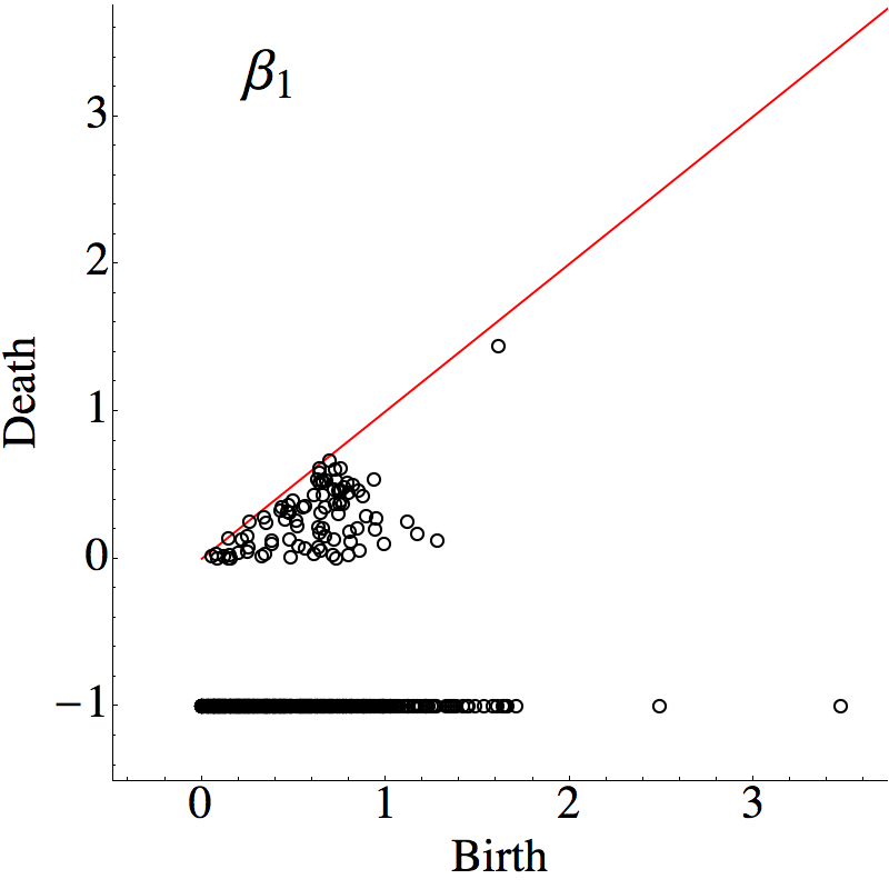
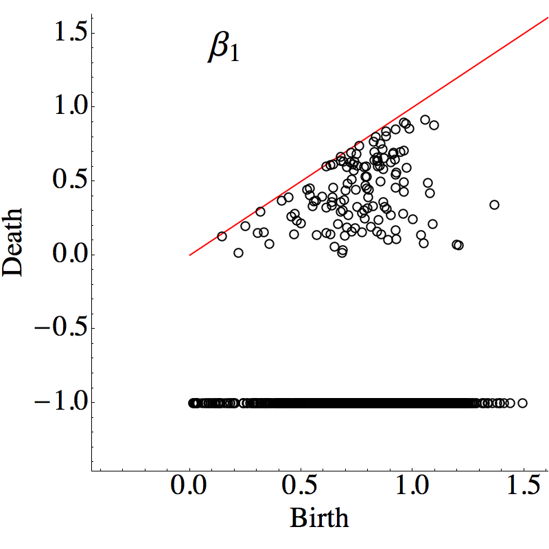
The defects region of the 1-dimension persistence diagrams provides additional information as explained in our paper.