
Lyapunov Function Computation
Overview
We consider the three-dimensional model considered by Cushing et. al. , given by
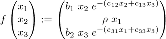
with parameters b1 = b2 = 5 , c12=c33=0.1 , c13=0.11 , c31=0.12 , ρ=0.8.
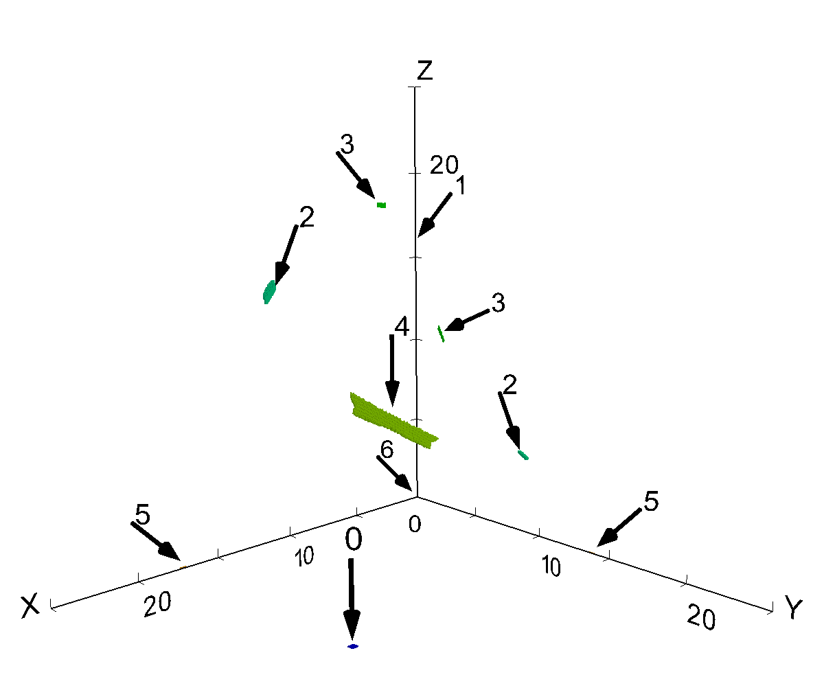
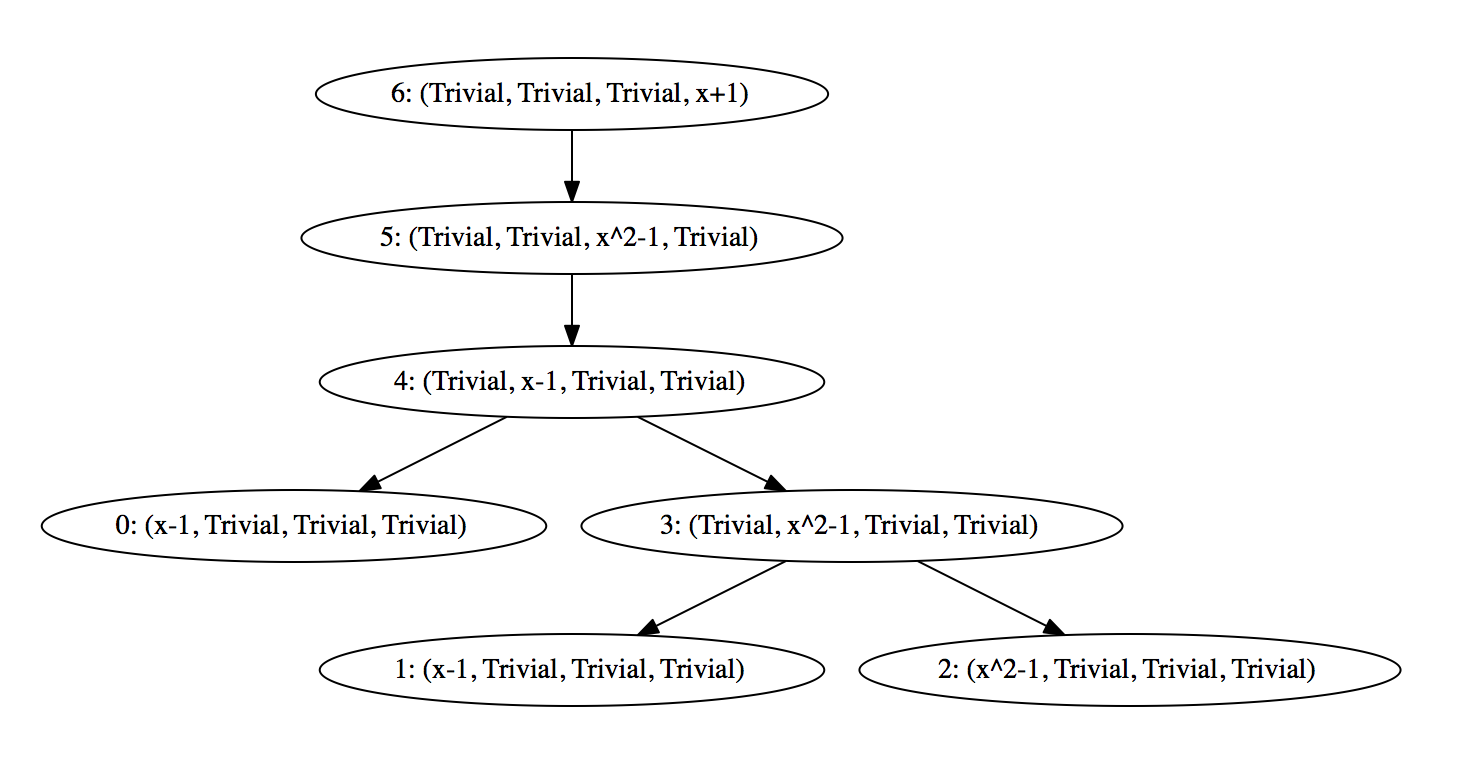
We first compute the Morse sets for this model using the Conley-Morse-Database software and obtain the Morse sets and the Conley-Morse graph below.
 |
 |
|---|---|
| a) 7 Morse Sets found for a level resolution of 34 | b) Conley-Morse graph |
 |
|---|
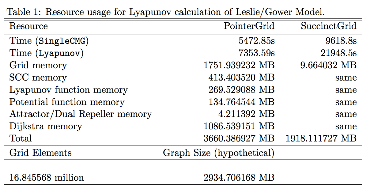
| c) Resource usage |
The Lyapunov function is computed using the program Lyapunov provided with the software and we give below a three-dimensional animation of the contours of the Lyapunov function.
Animation of the Lyapunov function contours.
We put together an animation showing the Morse sets and the Lyapunov function level curve going from 0 to 1.
Animation of the Lyapunov function level curves with the Morse sets.